Azure Cosmos DB – Partition and Throughput

In my previous article Introduction to Azure Cosmos DB, I mentioned Partition and Throughput only briefly. Adopting a good partition scheme is quintessential to setting up your Cosmos DB container for elastic scaling and blazing performance. This article will take a closer look at these two aspects to help fully utilize the storage and performance offerings of Cosmos DB.

Partition

Azure Cosmos DB containers store documents, graphs or tables. Containers (a.k.a. collections in the context of documents) are logical entities that could be distributed across multiple physical partitions or servers.

Physical and Logical Partitions

A physical partition is an internal Cosmos DB concept, essentially a fixed amount of SSD storage combined with a variable amount of compute power (CPU, memory and IO). The number of physical partitions of a container depends on its storage and throughput. For containers with shared throughput, number of partitions depends on RU/s assigned to the set of containers.

Request Unit (RU/s) – is the unit of throughput. 1 RU/s serves a get by self-link (internal property) or id of a 1 KB item.

When a collection is created, we can specify a fixed storage capacity of 10 GB or unlimited capacity. A fixed storage collection is limited in performance to a max of 10,000 RU/s. If we choose unlimited capacity, the collection created potentially has no max RU/s limit. Collections are supposedly unlimited in terms of storage and throughput, and physical partition management is handled by Cosmos DB behind the curtains. Note that for a multi-partition collection, we need to specify a partition key.

CosmosDB Container - Partitions

Data within a container having the same partition key value form a logical partition. The max storage limit of a logical partition is 10 GB, which means if data associated with a certain partition key value goes beyond 10 GB, the logical partition will be full and cannot grow any further. This is why adopting a good partition scheme is very important to avail the storage and performance guarantees of Azure Cosmos DB.

Partitioning example

Azure Cosmos DB internally has a limit for the max throughput that can be provided by a physical partition – PRUmax. This value keeps changing based on factors such as hardware used and platform upgrades. For now, keep in mind that this happens behind the scenes.

Let us assume PRUmax = 10,000 RU/s. We create an unlimited Collection product at 20,000 RU/s initial throughput and productid as the partition key. Cosmos DB has to create at least 2 physical partitions to support the 20,000 RU/s throughput requested. Currently, the default seems to be 5. So, Cosmos DB creates a new collection with 5 physical partitions. The throughput requested will be equally assigned to these physical partitions. This means, the max throughput limit for each partition is 20,000/5 = 4000 RU/s.

Partitioning-Example-Product collection

As we add new documents, Cosmos DB allocates the key space of partition key hashes evenly and consistently across the 5 physical partitions. If the partition key is well chosen, writes will be distributed evenly across the partitions, each partition serving nearly 5000 RU/s and a cumulative of nearly 20,000 RU/s. This is ideal. In real world, it is possible that we chose a bad partition key.

What can go wrong?

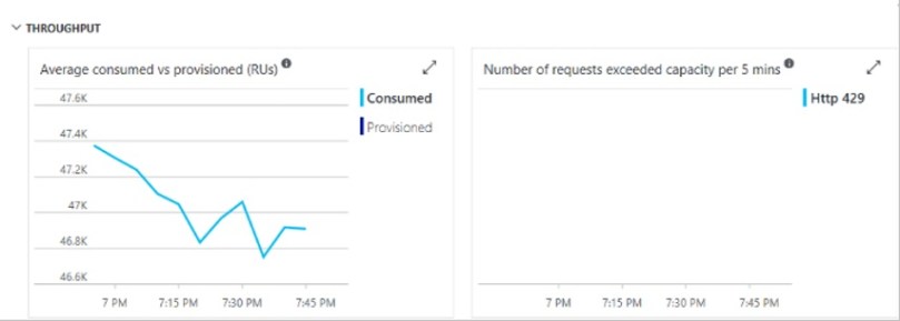
  • Performance impact: If majority of the concurrent writes/reads pertain to a specific partition key value, we could have 1 physical partition maxing out the 5000 RU/s allocated to it (hot partition), while the other 4 partitions idling. When this happens, requests are bound to get rate-limited and we will get Http 429 response code.
  • Storage impact: Earlier in the article, I mentioned the concept of logical partition. All data having the same partition key form a logical partition. Logical partitions cannot be split across physical partitions. For the same reason, if the partition key chosen is of bad cardinality, we could potentially have skewed storage distribution. Say, 1 logical partition becomes fatter faster and hits the max limit of 10 GB, while the others are nearly empty. The physical partition housing the maxed out logical partition cannot split and could thus cause an application downtime.

Physical partition split

Azure Cosmos DB manages physical partitions seamlessly behind the scenes, if you chose your partition key smartly that is. Following are two scenarios when Cosmos DB will split a physical partition.

  • Storage limit of 10 GB: When a physical partition is full, Cosmos DB will split it into 2 new partitions assigning data corresponding to nearly half of the keys to each new partition. As mentioned previously, the split cannot happen if data in the physical partition in question have the same partition key value.
  • Increasing throughput: When throughput assigned is increased such that the existing number of physical partitions are insufficient to support it, Cosmos DB will add new physical partitions. In the above example, if the throughput is increased to 100,000 RU/s, Cosmos DB would add 5 new physical partitions.
    Cosmos DB needs 100,000/PRUmax = 10 physical partitions to support the throughput setting.

Throughput

What makes Cosmos DB an attractive high volume transaction database is the ease of scaling. When request rates are low, throughput could be lowered to keep costs down. Cosmos DB’s performance is predictable. For example, a read of a 1-KB document with session consistency always consumes 1 RU, regardless of number of concurrent requests or amount of data stored.

There are, however, two major design considerations to facilitate elastic scaling of Azure Cosmos DB.

Distribute requests and storage

Ideal candidate property for partition key will allow writes to be distributed across various distinct values. Requests to the same partition key should remain lower than the max throughput limit allocated to a partition. A good partition key will evenly distribute writes across all physical partitions and not cause hot partitions. In our example, productid is a good partition key, because it is unlikely that all concurrent requests will be focused on a specific product. If we were to chose the property productcategory as partition key, that could potentially cause hot partitions

Partition scope for queries and transactions

At one extreme, we can use the same partition key for all documents. At the other extreme, we can have unique partition key for each document. Both approaches have their limitations. Using the same partition key for all documents will limit scalability and cause a hot partition and inefficient utilization of throughput. Using unique partition keys will support high scalability, but result in a lot of cross-partition queries and prevent use of cross-document transactions. Occasional fan-out of queries is not too bad, but frequent fan-out will incur high RU consumption and result in rate-limiting.

Estimating throughput

Throughput can be estimated based on the number of expected reads/writes per second. 1 Request Unit (RU) corresponds to read of a 1-KB document containing 10 unique property values by self-link or id. Write, replace or delete will consume more RU/s.

RU calculator

Microsoft provides a Request Unit calculator that serves to arrive at a base throughput to assign when creating a new collection. Be prepared to fine tune the RU setting as you trot along, but this is a good starting point.

This URL ignites nostalgia 🙂

Request Unit Calculator
Pic courtesy: Microsoft

Conclusion

Azure Cosmos DB is a lot more versatile compared to the initial Document DB days. With added support for Mongo DB, Graph, Cassandra and Table APIs and multi-master and global distribution support, Cosmos DB is definitely the most exciting product in database technology at the moment. With the new Azure data products such as Azure Stream Analytics, Azure Data Bricks and HDInsight supporting out-of-the-box integration with Cosmos DB, it is fast becoming a good candidate for Big Data solutions.

Please feel free to reach out if you have questions. I’m always happy to discuss technology 🙂

Introduction to Azure Cosmos DB

What is Azure Cosmos DB?

Cosmos DB started as an internal project – “Project Florence” – at Microsoft in 2010. It is a globally distributed, highly scalable and performant multi-model database service built on Azure. It was built ground up with horizontal scalability and global distribution in view, so you can expect seamless geo-replication to Azure regions by clicking on a map and performance to the order of milliseconds.

CosmosDBIcon

Why should you use Cosmos DB?

Cosmos DB is the future of storage. Below are some reasons you may want to use it.

  • You use Microsoft stack already and find your favourite RDBMS – SQL Server – too slow
  • Your applications need to process large amounts of data at blazing speeds
  • Your data is not relational anymore, you want to use JSON document store or Graph DB or one of the many popular APIs Cosmos DB supports
  • Big Data applications – This is an evolving use case. Many Azure products such as Azure Stream Analytics, HDInsight and Data Bricks integrate with Cosmos DB, making it an ideal choice for persisting big data.
  • You are having to “over-provision” specs to cover peak loads on the database server
  • Your business spans multiple continents and you want easy and reliable replication
  • You trust Microsoft to do a better job with availability using Azure

CosmosDBGeoReplication

Hello Collections!

Collections are to Cosmos DB what tables are to an RDBMS. This analogy is for easy understanding; don’t get hung up on details. There are many differences between collections and tables. A more generic term is Container, especially as Cosmos DB has evolved to support more APIs since the Document DB days.

After you create a Database in your Cosmos DB account, you can create your first collection. Below are a few aspects of a collection you need to be familiar with.

1Request Units / Throughput: Request Unit (RU) is the currency of Cosmos DB.

1 RU = capacity to read* a single 1 KB item consisting of 10 unique property values
*by self-link or id

A collection need not be a set of documents of the same schema. As Cosmos DB is schema-agnostic, you can very well store different document types in the same collection. That said, you may want to store document types that need the same amount of scalability and storage in the same collection. Cosmos DB is cost effective for high volume transaction systems because RU/s for a collection can be ramped up at peak hours and reduced to a minimum during hours of low trade.

When the provisioned number of RU/s is used up, client requests may experience throttling. Prolonged throttling indicates an insufficient throughput setting.

CosmosDBThroughput

2. Partition: Each document in a collection has a partition key and an id

Partition key helps to identify the logical partition, and the id field helps to identify a specific document.

When you create a collection with an initial throughput more than 1000 RU/s, the resulting collection has unlimited scalability. Depending on the initial throughput assigned, Cosmos DB computes the number of physical partitions required to support the provisioned throughput. Logical partitions have a storage limit of 10GB. Due to this, a single logical partition (housing documents having a certain partition key value, such as Product Type = ‘Motorbike helmet’) should not amount to more than 10GB. Theoretically, the number of partitions in a collection can be infinite. Therefore, a good partition key must be a field having a suitable cardinality. With a bad partition key, you are bound to have uneven distributions of data and are likely to hit the 10 GB storage limit per partition.

CosmosDBPartitions3. Time to Live: TTL can be set at a collection or document level. Document level TTL takes precedence, obviously.

Simply put, if TTL for a document is set to 3600 seconds, the document expires when it is older than 3600 seconds. System field _ts (_ts or timestamp is set to Epoch time) indicates the last modified time of a document. Be careful when you set this at collection level. However, this feature helps to implement a sound purge policy.

Global Distribution:

Geo-replication becomes as simple as clicking on a graph with Cosmos DB’s global distribution feature. With more than 50 Azure regions, you could not only set multiple Read regions for global customers, but also specify several failover regions to help with disaster recovery.

CosmosDBAutomaticFailover

There is a lot more to Cosmos DB than can be covered in a single post. With a whole heap of new Azure features that it can easily integrate with, such as SQL Managed Instance, SQL Data warehouse, HDInsight, Data bricks and Data lakes, Cosmos DB is here to stay.

Check out my post about Cosmos DB migration tool if you are migrating data to or from Cosmos DB.

Export data from Cosmos DB to SQL Server

Cosmos DB is Microsoft’s latest NoSQL database offering low latency, high scalability and geo-distribution to any Azure region. Read Microsoft documentation about Cosmos DB here or check out my blog about Introduction to Azure Cosmos DB. In its infancy, Cosmos DB was known as Document DB. Renaming was inevitable as Document DB evolved beyond just a document store.

Following is a simple note on how to export data from Cosmos DB to SQL Server. You may want a dump of data from a Cosmos DB collection to SQL Server for analysis, data integrity checks, troubleshooting a production issue or to derive insights. If you want to set up a real-time data pipeline from Cosmos DB to SQL Server, check out this post: – https://sqlroadie.wordpress.com/2019/07/21/azure-cosmos-db-real-time-data-movement-using-change-feed-and-azure-functions/

There are a few methods to export data from Cosmos DB. The quickest one is to use Document DB / Cosmos DB Migration Tool. This is a tool provided by Microsoft  to migrate data TO/FROM various sources such as MongoDB, JSON, csv and SQL Server to Cosmos DB.

1. Use Azure Cosmos DB Migration tool to export data to json files:

  • Install the tool and launch as Administrator (use an Azure VM for best performance). Please be mindful of spike in RU costs when exporting data from your collection. To avoid throttling, scale your collection up as required just before you do the export or export in off-peak hours, if any.  Leave a comment if you need any pointer on this.LaunchCosmosDBMigrationTool
  • Choose source – DocumentDB (CosmosDB aka DocumentDB)

CosmosDBMigrationTool-Source

  • Specify connection string. You can find endpoint and key from Keys section of your CosmosDB account in Azure portal. Please note that CosmosDB is case-sensitive.

CosmosDBMigrationTool-ConnectionString

  • A peek into Advanced options
    • Include internal fields – for each document, Cosmos DB maintains a set of auto-generated internal/system fields such as _ts and _self. Their names start with an underscore, making it easy to differentiate them from user fields. This option lets you include internal fields in the output. This is handy, especially the _ts field, which indicates when the document was last updated.
    • Number of retries on failure & Retry interval – Set a reasonable number of retries. In this case, I have used the value 1.
    • Connection Mode you want to use Gateway to get best performance and to bypass firewall rules.

CosmosDBMigrationTool-AdvancedOptions

  • Specify target information. In this case, we want to export to a json document. We could either output to a local file or a blob.

CosmosDBMigrationTool-TargetInformation

  • Error Logging. Set these options to enable error logging.

CosmosDBMigrationTool-ErrorLogging

Hit Import and if there are no errors, you will soon have a new json file with all the data from your collection. If you want only a subset of data, all you need to do is modify your source query.

2. Import json files to SQL Server:

SQL Server 2016 introduced a JSON parse function called OPENJSON. If none of your user databases are upgraded to 2016 yet, but you have a 2016 engine, context-switch to a system database to use OPENJSON.

DECLARE @productNutrition varchar(max);

--Read from the json file using openrowset
SELECT @productNutrition = BulkColumn
FROM OPENROWSET(BULK'C:\Users\Smruthi\Downloads\Arjun\productnutrition_20180427.json', SINGLE_BLOB) JSON;

--Pass the variable containing json as parameter to OPENJSON function
SELECT *
FROM OPENJSON (@productNutrition)
WITH
(
ProductID varchar(20) '$.id',
ProductDescription varchar(100) '$.description',
ProductGroup varchar(200) '$.foodGroup',
ServingAmount float '$.servings[1].amount',
ServingUnit varchar(10) '$.servings[1].description',
nutrients nvarchar(max) as json --note that json is case sensitive
)

Give it a go yourself. If you have any question, leave a comment and I will be happy to assist.

If you are exploring Cosmos DB, consider reading my blog about Azure Cosmos DB – Partition and Throughput to get an overview of partitioning and scaling concepts.

jsonfileSample

openjson Example

Live Query Statistics – SQL Server 2016

SQL Server Management Studio (SSMS) 2016 has a handy new feature to View Live Query Statistics. This feature also works when connected to a 2014 instance using SSMS 2016.

Why use it?

Previously, similar stats were available by doing so:

SET STATISTICS "Detail" ON;

With the new feature, the main difference is that as the query progresses, stats are refreshed, thus providing a live coverage of what SQL Server is up to. This is a fantastic feature to learn about query processing and execution plans, and it helps to identify performance problems. Only yesterday, I used it to identify a “bad plan” where SQL was doing an Eager Spool by cross-joining two million record tables, and thus filling tempdb.

How to use it?

To use the feature, simply click on “Include Live Query Statistics” button in the toolbar or under menu Query -> Include Live Query Statistics.
IncludeLiveQueryStatistics-SQLServer2016

Watch the magic unfold when you execute query.

LiveQueryStatistics-Example.png


If you are not using SQL Sentry Plan Explorer already, please install PRO version for free from Sentry One. I find it amazing and it’s probably the best free tool out there to do performance analysis. Install the SSMS add-in, and you can right click on plan and view plan in SQL Sentry Plan Explorer. It becomes incredibly useful for complex plans that are cumbersome to navigate in SQL Server. Not to mention the host of other info that’s presented nicely to make performance tuning enjoyable.

SQLSentryPlanExplorer-AddIn

SQLSentryPlanExplorer.jpg

Watch out for that..

Live Query Statistics is an interesting feature, but I had a nervous few moments when my long-running ETL stored procedure began to produce a plan that was way too big for SSMS to handle. I had to eventually cancel execution and view plan from DMV. So, while it is a nice feature, watch out for a few gotchas. Microsoft also advises that there might be a mild performance dip in execution of your query when you are using this feature.

Who can use it?

You need to have SHOWPLAN and VIEW SERVER STATE permissions to be able to use this feature effectively.

Overall, this is a great feature that makes information available at finger tips when you are possibly scrambling to address that performance issue that is driving everyone nuts!

Database Mail shutting down. Mail queue has been stopped.

DB mail in our production servers started acting up last week. We have SQL Server 2012 SP1. There were a couple of sets of symptoms. Following is what I did to get DB mail working again.

I hope you don’t spend 4 hrs like me to find a solution.

Symptom 1:

Mails will not be sent anymore. Sending test mail will not work.  When DB mail status is checked using the following SP, it will return “STARTED”.

USE msdb
GO
EXEC dbo.sysmail_help_status_sp

However, checking the status of mail items themselves using the following SP will show that they are “unsent”.

SELECT TOP 10 sent_status, *
FROM dbo.sysmail_allitems WITH(NOLOCK READUNCOMMITTED)
ORDER BY send_request_date desc

Stopping DB mail using the following SP does not work anymore. The command takes forever to execute and nothing happens.

USE msdb
GO
EXEC dbo.sysmail_stop_sp

If these are the symptoms,

  1. Kill the process “DatabaseMail.exe” from task manager of the server to stop DB mail.
  2. Check status using sysmail_help_status_sp and ensure it shows “STOPPED”.
  3. Start DB mail using the following command.
    USE msdb
    GO
    EXEC dbo.sysmail_start_sp
  4. Check status of mail items. The sent_status column should now show “sent”.

Symptom 2:

Fix for “Symptom 1” worked on one server, but on another, mails were not being sent at all. If the above fix doesn’t do it for you, Stop DB mail and check mail log in SSMS at

Management->Database Mail->View Database Mail Log

If log shows the message – “DatabaseMail process is shutting down. Mail queue has been stopped”, check for mails stuck in the mail queue.

Use msdb
GO
Select count(*) from ExternalMailQueue – Check if this is non-zero
  1. If the above query returns a non-zero number, there are stuck mails. Use following script to remove all items from the queue. Please be informed that all these MAILS WILL BE LOST!
Use msdb
GO
ALTER QUEUE ExternalMailQueue WITH STATUS = ON
set nocount on
declare @Conversation_handle uniqueidentifier;
declare @message_type nvarchar(256);
declare @counter bigint;
declare @counter2 bigint;
set @counter = (select count(*) from ExternalMailQueue)
set @counter2=0
while (@counter2<=@counter)
begin
receive @Conversation_handle = conversation_handle, @message_type = message_type_name from ExternalMailQueue
set @counter2 = @counter2 + 1
end

2. Check number of mails in the mail queue. It will be zero.

Use msdb
GO
Select count(*) from ExternalMailQueue

3. Start DB mail using

USE msdb
GO
EXEC dbo.sysmail_start_sp

 4. Check status of mail items. The sent_status column should now show “sent”.

XQuery

In 2005 version of SQL Server, XQuerying was introduced. It’s a powerful feature and when used together with a CTE, it helps to keep code simple and clean. I use XML extensively in my code and many a time, I find myself looking up code, searching the internet or trying things out myself. I hope this post will be a single point of reference to most of the usual XQuery coding.

Following is a simple script to read from an XML variable. Same code can be used to read from an XML column as well.

NOTE: I will append more XQuery code samples to this post.

DECLARE @xmlProduct XML = 
'<Catalog>
	<Product>
		<Name>Selle Italia Road</Name>
		<Code>SIR-1</Code>
		<Category>Saddle</Category>
		<Description>Sleek saddle from Selle Italia</Description>
		<UnitPrice>50</UnitPrice>
		<Currency>USD</Currency>
	</Product>
	<Product>
		<Name>Brooks Tourer</Name>
		<Code>BT-T</Code>
		<Category>Saddle</Category>
		<Description>Brooks leather saddle for touring</Description>
		<UnitPrice>120</UnitPrice>
		<Currency>USD</Currency>
	</Product>
</Catalog>
'
--Read from nodes
SELECT
c.value('Name[1]','varchar(50)') [ProductName],
c.value('Code[1]','varchar(50)') [Code],
c.value('Category[1]','varchar(50)') [Category],
c.value('UnitPrice[1]','varchar(50)') + CHAR(32) + c.value('Currency[1]','varchar(50)') [Price],
c.value('Description[1]','varchar(50)') [Description]
FROM 
@xmlProduct.nodes('//Catalog/Product') AS TAB(c)

Output:
XQueryOutput

Retrieve unsaved query

I was working on a remote machine and while I was away, the machine was restarted. Lost the scripts I had not saved, or so I thought; and then I came up with this – was a life saver!

SELECT TOP 10 
EST.text
FROM sys.dm_exec_query_stats EQS
CROSS APPLY sys.dm_exec_sql_text(eqs.sql_handle) EST
WHERE EST.text LIKE '%text%'
ORDER BY last_execution_time DESC

Find tables which are most commonly used in Stored Procedures

When you start working on a new project, one of the important tasks as a database developer is to get used to the table names. Here’s a script which will help you identify the most commonly used tables (assuming that the most commonly used are the most important).

SELECT TOP 50
t.name, COUNT(1) tcount
FROM INFORMATION_SCHEMA.routines r
INNER JOIN sys.tables t ON r.ROUTINE_NAME LIKE ('%' + t.name + '%')
GROUP BY t.name 
ORDER BY tcount desc