Azure Cosmos DB: real-time data movement using Change Feed and Azure Functions

July 21, 2019September 26, 2019 Arjun13 Comments

Many people who read my Cosmos DB articles are looking for an effective way to export data to SQL, either on-demand or in real-time. After performing a search term analysis for my blog earlier this year, I had made up my mind about posting a solid article on exporting data from Cosmos DB to SQL Server.

Note that this serverless and event-based architecture may be used to not only persist Cosmos DB changes to SQL Server, but trigger alternate actions such as stream processing or loading to blob/Data Lake.

Real-time ETL using Cosmos DB Change Feed and Azure Functions

In this article, we will focus on creating a data pipeline to ETL (Extract, Transform and Load) Cosmos DB container changes to a SQL Server database. My main requirements or design considerations are:

Fault-tolerant and near real-time processing
Incur minimum additional cost
Simple to implement and maintain

Cosmos DB Change Feed

Cosmos DB Change Feed listens to Cosmos DB containers for changes and outputs the list of items that were changed in the chronological order of their modification. Cosmos DB Change Feed enables building efficient and scalable solutions for the following use cases:

Triggering a notification or calling an API
Real-time stream processing
Downstream data movement or archiving

Types of operations

Change feed tracks inserts and updates. Deletes are not tracked yet
Cannot control change feed to track only one kind of operation, for example only inserts
For tracking deletes in the Change Feed, workaround is to soft-delete and assign a small TTL (Time To Live) value of “n” to automatically delete the item after “n” seconds
Change Feed can be read for historic items, as long as the items have not been deleted
Change Feed items are available in order of their modification time (_ts system attribute), per logical partition key, and tagged with the same _lsn (system attribute) value for all items modified in the same transaction

Read more about Azure Cosmos DB Change Feed from Microsoft docs to gain a thorough understanding. Change Feed can be processed using Azure Functions or Change Feed Processor Library. In this article, we will use Azure Functions.

Azure Functions

Azure Functions is an event-driven, serverless compute platform for easily running small pieces of code in Azure. Key points to note are:

Write specific code for a problem without worrying about an application or the infrastructure to run it
Use either C#, F#, Node.js, Java, or PHP for coding
Pay only for the time your code runs and trust Azure to scale
As of July 2019, the Azure Functions trigger for Cosmos DB is supported for use with the Core (SQL) API only

Read more from Microsoft docs to understand full capabilities of Azure Functions.

If you use Consumption plan pricing, it includes a monthly free grant of 1 million requests and 400,000 GBs of resource consumption per month per subscription in pay-as-you-go pricing across all function apps in that subscription, as per MS docs.

Compare hosting plans and check out pricing details for Azure Functions at the Functions pricing page to gain a thorough understanding of pricing options.

Real-time data movement using Change Feed and Azure Functions

The following architecture will allow us to listen to a Cosmos DB container for inserts and updates, and copy changes to a SQL Server Table. Note that Change Feed is enabled by default for all Cosmos DB containers.

I will create a Cosmos DB container and add an Azure Function to listen to the Cosmos DB container. I will then modify the Azure Function code to parse modified container items and save them to a SQL Server table.

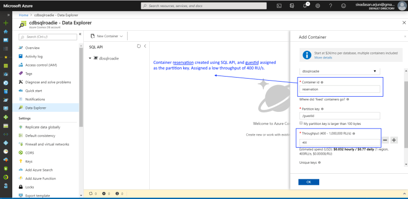
1. First, I navigated to Azure portal, Cosmos DB blade and created a container called reservation in my Cosmos DB database. As it is purely for the purposes of this demo, I assigned lowest throughput of 400 RU/s

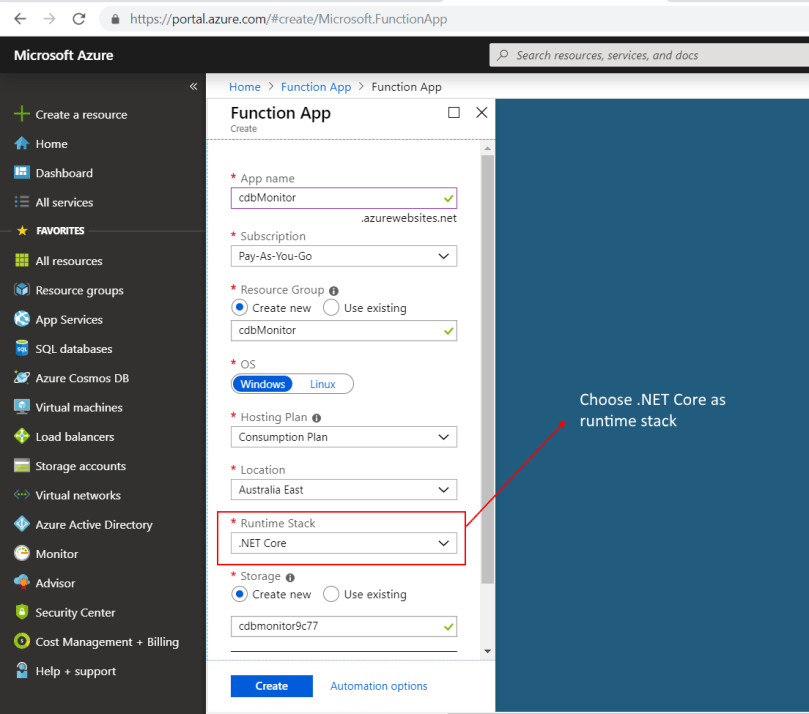
2. Now that the container is ready, proceed to create an Azure Function App. The Azure Function will be hosted in the Azure Function app

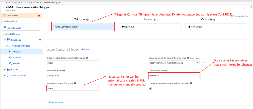
3. Add an Azure Function within the newly created Azure Function App. Azure Function trigger for Cosmos DB utilizes the scaling and event-detection functionalities of Change Feed processor, to allow creation of small reactive Azure Functions that will be triggered on each new input to the Cosmos DB container.

4. Configure the trigger. Leases container may be manually created. Alternately, check the box that says “Create lease collection if it does not exist”. Please note that you would incur cost for storage and compute for leases container.

I got this error that read – “The binding type(s) ‘cosmosDBTrigger’ are not registered. You just need to install the relevant extension. I saw many posts about this, so it will most likely be fixed soon.

Sort out the error by installing the extension for Azure Cosmos DB trigger.

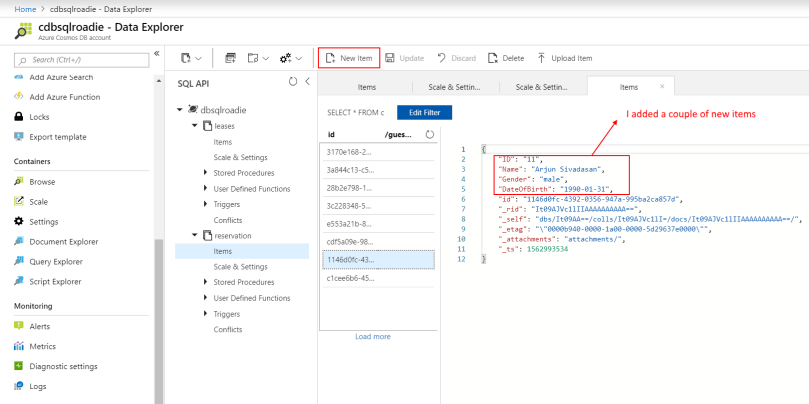
5. Once the function is up and running, add an item to the reservations container that we are monitoring. And we have a working solution!

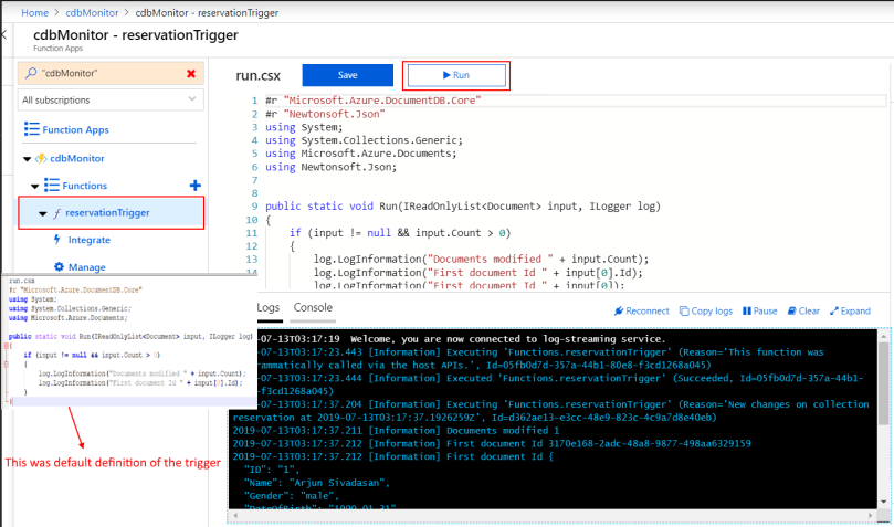
6. Trigger definition may be modified to achieve different things, in our case we will parse the feed output and persist changes to SQL server. You can download the csx file I used.

Summary

We have successfully implemented a serverless, event-based low cost architecture that is built to scale. Bear in mind that you would still end up paying for Azure Function and the underlying leases collection, but there will be minimum additional RU cost incurred from reading your monitored container(s) as you are tapping into the Change Feed.

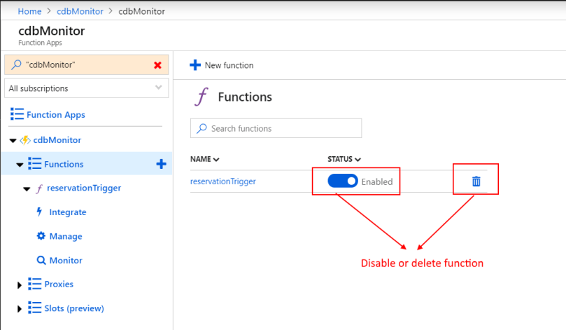
You can monitor the function and troubleshoot errors.

I hope you found the article useful. Add a comment if you have feedback for me. If you have any question, drop me a line on LinkedIn. I’ll be happy to help 🙂 Happy coding!

Resources:

https://docs.microsoft.com/en-us/azure/cosmos-db/change-feed
https://docs.microsoft.com/en-us/azure/cosmos-db/changefeed-ecommerce-solution
https://azure.microsoft.com/en-au/services/functions/
https://docs.microsoft.com/en-us/azure/azure-functions/functions-overview
https://docs.microsoft.com/en-us/azure/azure-functions/functions-bindings-cosmosdb-v2
https://docs.microsoft.com/en-us/azure/cosmos-db/change-feed-functions
https://azure.microsoft.com/en-au/resources/videos/azure-cosmosdb-change-feed/
https://h-savran.blogspot.com/2019/03/introduction-to-change-feed-in-cosmos.html

Demo: Predictive Modeling using R and SQL Server Machine Learning Services

May 29, 2019May 29, 2019 ArjunLeave a comment

Late last year, I wrote a series of articles about Predictive Modeling using R and SQL Server Machine Learning Services. At the time, I thought MLS was an underutilized feature of SQL Server. With a view to sharing my learning on the topic, I presented a session at the local SQL Server User Group earlier this month.

Presentation

MLS at QLD SQL Server User Group

This article will be focused on content presented at the User Group meeting. Below is the presentation I put together. If you are new to Machine Learning on premises, it will help you understand the capabilities of this powerful feature of SQL Server.

Demo

As a typical data nerd, I was more excited about the demo than the session itself. For the demo, I chose to predict heart disease risk using the popular heart disease data set from UCI.

https://archive.ics.uci.edu/ml/machine-learning-databases/heart-disease/processed.cleveland.data

https://archive.ics.uci.edu/ml/machine-learning-databases/heart-disease/heart-disease.names

Using R, a predictive model is trained and tested against known results.
After testing and comparing a few Machine Learning models, the R scripts were wrapped in SQL Server Stored Procedures letting us execute R scripts through Stored Procedures
The trained models were stored in a SQL Server table, and were used to perform Machine Learning predictions through Stored Procedure calls
Last step in the demo covered Native Scoring using the native C++ extension capabilities in SQL Server 2017

Demo solution is available for download at https://github.com/sqlroadie/PredictiveModelingUsingRandSQLServerMLS

Solution contains the following files:

heart-disease.data – UCI dataset attached for reference heart-disease.names – Data description. Go through this file to understand what the variables mean
PredictiveModelingUsingR.r – R script (with comments wherever applicable) that builds the predictive Model using RevoScaleR package. Go through this to understand how the models are created and used for prediction.
PredictiveModelingUsingMLS.sql – SQL script that uses R code covered in the previous file to build a Machine Learning predictive model that is executed in the SQL on premises instance

Predictive Modeling using R and SQL Server Machine Learning Services

If you need a hand with the demo, please drop me a note. LinkedIn is the best way to get in touch with me. Happy learning!

Thanks to Wardy IT and their Marketing Manager, Michaela Murray, for their continued efforts on organizing the user group meetings.

Analyzing Heart Disease risk using Key Influencers AI visual in Power BI

February 23, 2019March 10, 2019 Arjun7 Comments

The Gartner Magic Quadrant for 2019, announced earlier this month, names Microsoft the leader in Analytics and Business Intelligence Platforms. Microsoft also coincidentally announced the public preview release of its first AI-driven visual for Power BI – Key Influencers – this month, among a number of new features for Feb 2019. Inbuilt integration of Power BI with many Azure data products would catapult Power BI miles ahead of Tableau in the long run.

Key Influencers is the first of many AI visuals Microsoft would release I assume, in their efforts to democratize AI and make their customers look cool 🙂 In this article, we will go over the various features of this new visual using a publicly available dataset, and get familiar with interpreting the results. Download a copy of Power BI Desktop file for the example I am using in this article and try it out yourself using the free Power BI Desktop tool.

Key Influencers

Key Influencers is a powerful Power BI visual that lets us understand the factors that drive a metric. Power BI analyzes data, ranks the factors that matter, and displays them as key influencers. Under the hood, Power BI uses ML.NET to run logistic regression to calculate the key influencers. Logistic regression is a statistical model that compares different groups to each other, also taking into consideration the number of data points available for a factor.

As the visual is still in preview, there are a number of limitations. My first attempt to use Key Influencers using a survey responses dataset was rather unimpressive.

In my second attempt, I used the popular Heart Disease dataset from UCI to identify key influencers affecting heart disease, and achieved good results.

Heart Disease - Key Influencers Power BI.jpg

Limitations

Before we delve any further, let us take a look at the limitations that apply in the public preview phase of the visual. Pay attention here to avoid frustration as you explore the visual.

Following features are not supported:

Analyzing metrics that are aggregates/measures
Direct Query / Live Connection / Row Level Security – support
Consuming the visual in Power BI Embedded and Power BI mobile apps

Using the Key Influencers Visual

As a first time user, I found the Key Influencers visual intuitive and self-explanatory. It hardly takes a few minutes to set up the visual once you have clean data. Check out Microsoft documentation to understand all aspects of the visual. You could also download a copy of Power BI Desktop file for the example I am using in this article.

Note: Keep column names readable as this will help interpret the visual better

Getting Familiar

There are 2 tabs available within the visual – Key influencers and Top Segments.

The Key influencers tab displays the key factors affecting the metric value selected. In this case, the top factor that affects positive diagnosis of Heart Disease, based on our dataset, is Reversible Defect Thalassemia – increasing the risk of heart disease by 2.83 times when the value of Reversible Defect Thalassemia is 7.

On the right hand side, there is a column chart showing distribution of the selected factor. The check box at the bottom lets you display only influential factor values. We could click-select a different factor to see how it contributes to heart disease.

Heart Disease - Key Influencers Power BI - Getting Familiar.jpg

The Top segments tab displays different segments identified by Power BI within the population, for the metric value selected. Click-select a segment to view more details such as the factor values that define the segment, and how the segment compares against the average. We could also drill down further into the segment to split by additional fields.

Under the hood, Power BI uses ML.NET to run a decision tree to find interesting subgroups. The objective of the decision tree is to end up with a subgroup of datapoints that is relatively high in the metric we are interested in – in our case, the patients who are suspected to have heart disease.

Heart Disease - Key Influencers Power BI - Top Segment.jpg

Heart Disease - Key Influencers Power BI - Top Segment Details.jpg

First Impression

Considering that it is still in preview and is only going to get better, Key Influencers ticks the right boxes. The rationale behind choosing a popular dataset, such as the Heart Disease dataset from UCI, for my example was to allow for comparison of results to Machine Learning models that are already publicly available. Power BI seems to identify influencers correctly and does a good job at presentation. I’m thoroughly impressed by this new feature.

Resources:

Download the Power BI workbook used in the example – https://drive.google.com/open?id=13Pt25UPt7dOW3raZmavHHVl7gAStv5uy
Intro to Key Influencers by Microsoft: https://docs.microsoft.com/en-us/power-bi/visuals/power-bi-visualization-influencers
Power BI Feb 2019 feature summary – https://powerbi.microsoft.com/en-us/blog/power-bi-desktop-february-2019-feature-summary/

Heart Disease Data source
Donor: David W. Aha (aha ‘@’ ics.uci.edu) (714) 856-8779
Creators:

Hungarian Institute of Cardiology. Budapest: Andras Janosi, M.D.
University Hospital, Zurich, Switzerland: William Steinbrunn, M.D.
University Hospital, Basel, Switzerland: Matthias Pfisterer, M.D.
V.A. Medical Center, Long Beach and Cleveland Clinic Foundation: Robert Detrano, M.D., Ph.D.

Azure Databricks – Introduction (Free Trial)

February 17, 2019February 23, 2019 Arjun

Microsoft’s Azure Databricks is an advanced Apache Spark platform that brings data and business teams together. In this introductory article, we will look at what the use cases for Azure Databricks are, and how it really manages to bring technology and business teams together.

Databricks

Before we delve deeper into Databricks, it is good to have a general understanding of Apache Spark.

Apache Spark is an open-source, unified analytics engine for big data processing, maintained by the Apache Software Foundation. Spark and its RDDs were developed in 2012 in response to limitations of MapReduce.

Key factors that make Spark ideal for big data processing are:

Speed – up to 100X faster
Ease of use – code in Java, Scala, Python, R and SQL
Generality – use SQL, streaming and complex analytics

Apache Spark Ecosystem.jpg — Pic courtesy: Microsoft

Databricks – the company – was founded by creators of Apache Spark. Databricks provides a web-based platform for working with Spark, with automated cluster management and IPython-style notebooks. It is aimed at unifying data science and engineering across the Machine Learning (ML) life cycle from data preparation, to experimentation and deployment of ML applications. Databricks, by virtue of its big data processing capabilities, also facilitates big data analytics. Databricks, as the name implies, thus lets you build solutions using bricks of data.

Azure Databricks

Azure Databricks combines Databricks and Azure to allow easy set up of streamlined workflows and an interactive work space that lets data teams and business collaborate. If you’ve been following data products on Azure, you’d be nodding your head along, imagining where Microsoft is going with this 🙂

Azure Databricks enables integration across a variety of Azure data stores and services such as Azure SQL Data Warehouse, Azure Cosmos DB, Azure Data Lake Store, Azure Blob storage, and Azure Event Hub. Add rich integration with Power BI, and you have a complete solution.

Azure Databricks Overview — Pic courtesy: Microsoft

Why use Azure Databricks?

By now, we understand that Azure Databricks is an Apache Spark-based analytics platform that has big data processing capabilities and brings data and business teams together. How exactly does it do that, and why would someone use Azure Databricks?

Fully managed Apache Spark clusters: With the serverless option, create clusters easily without having to set up your own data infrastructure. Dynamically auto-scale clusters up and down, and auto-terminate inactive clusters after a predefined period of inactivity. Share clusters with your teams, reduce time spent on infrastructure management and improve iteration time.
Interactive workspace: Streamline data processing using secure workspaces, assign relevant permissions to different teams. Mix languages within a notebook – use your favorite out of R, Python, Scala and SQL. Explore, model and execute data-driven applications by letting Data Engineers prepare and load data, Data Scientists build models, and business teams analyze results. Visualize data in a few clicks using familiar tools like Matplotlib, ggplot or take advantage of the rich integration with Power BI.
Enterprise security: Use SSO through Azure Active Directory integration to run complete Azure-based solutions. Roles-based access control enables fine-grained user permissions for notebooks, clusters, jobs, and data.
Schedule notebook execution: Build, train and deploy AI models at scale using GPU-enabled clusters. Schedule notebooks as jobs, using runtime for ML that comes preinstalled and preconfigured with deep learning frameworks and libraries such as TensorFlow and Keras. Monitor job performance and stay on top of your game.
Scale seamlessly: Target any amount of data or any project size using a comprehensive set of analytics technologies including SQL, Streaming, MLlib and GraphX. Configure number of threads, select number of cores and enable autoscaling to dynamically scale processing capabilities leveraging a Spark engine that is faster and performant through various optimizations at the I/O layer and processing layer (Databricks I/O).

Of course, all of this comes at a price. If this article has piqued your interest, hop over to Azure Databricks homepage and avail the 14 day free trial!

Azure Databricks - Free Trial 14 days.jpg

Suggested learning path:

Read more about Azure Databricks – https://docs.microsoft.com/en-us/azure/azure-databricks/what-is-azure-databricks
Create a Spark cluster and run a Spark job on Azure Databricks – https://docs.microsoft.com/en-us/azure/azure-databricks/quickstart-create-databricks-workspace-portal#clean-up-resources
ETL using Azure Databricks – https://docs.microsoft.com/en-us/azure/azure-databricks/databricks-extract-load-sql-data-warehouse
Stream data into Azure Databricks using Event Hubs – https://docs.microsoft.com/en-us/azure/azure-databricks/databricks-stream-from-eventhubs
Sentiment analysis on streaming data using Azure Databricks – https://docs.microsoft.com/en-us/azure/azure-databricks/databricks-sentiment-analysis-cognitive-services

I hope you found the article useful. Share your learning experience with me. My next article will be on Real-time analytics using Azure Databricks.

Azure Databricks - Real time analytics.jpg — Azure Databricks

Resources:

https://azure.microsoft.com/en-au/services/databricks/
https://databricks.com/product/azure
https://docs.microsoft.com/en-us/azure/azure-databricks/what-is-azure-databricks
https://docs.microsoft.com/en-us/azure/azure-databricks/quickstart-create-databricks-workspace-portal#clean-up-resources
https://databricks.com/blog/2019/02/07/high-performance-modern-data-warehousing-with-azure-databricks-and-azure-sql-dw.html

Part 2: Predictive Modeling using R and SQL Server Machine Learning Services

November 18, 2018November 18, 2018 Arjun2 Comments

Recap!

Part 1 of Predictive Modeling using R and SQL Server Machine Learning Services covered an overview of Predictive Modeling and the steps involved in building a Predictive Model. Using our sample dataset – Ski Resort rental data – we wanted to predict RentalCount for the year 2015, given the variables – Month, Day, Weekday, Holiday and Snow.

Part 1 covered:
– Getting data from a SQL Server database
– Preparing data for modeling
– Training models
– Comparing results and finalizing a model

We found that for this problem, predictions using the Decision Tree model were more accurate than the Linear Regression model. SQL Server Machine Learning Services (MLS) lets us train and test Predictive Models using R or Python, in the context of SQL Server. Thus, we can build T-SQL programs that contain embedded R/Python scripts that train on data stored in the database.

Deploy Machine Learning code with SQL Server

In this part, we will deploy the R code we wrote in Part 1 to SQL Server. To deploy, we will store the trained model in database and create a stored procedure that predicts using the model. This stored procedure can be invoked from applications.

1. Create Table for storing the model: Here, we create a table in SQL Server to store the trained model. The model will be used for prediction in step 3.

2. Create Stored Procedure for generating the model: This stored procedure will use the R scripts we wrote in Part 1 utilizing sp_execute_external_script introduced in SQL Server 2016. To execute sp_execute_external_script, first enable external scripts by using the statement – sp_configure ‘external scripts enabled’, 1;

The function to generate Decision Tree model – rxDTree – is part of the RevoScaleR package for R. RevoScaleR package includes numerous other R functions for importing, transforming, and analyzing data at scale. Point to note is that the functions run on the RevoScaleR interpreter, built on open-source R. It is engineered to leverage the multithreaded and multinode architecture of the host platform, meaning when R code executes within a SQL Server SP, it utilizes parallel processing.

2002_SPToGenerateTrainedDTreeModel

3. Create Stored Procedure for prediction: Now that we have the model output, we can create an SP that would use the model to predict rental count for new data. Again, we are using the R code covered in Part 1, only that this time we are using it in a SQL Stored Procedure.

Isn’t that just awesome? We have a Predictive Model that can be used within applications to predict rental count. Now that we have covered a sample project, in Part 3 of the series, I will share my experience using SQL Server Machine Learning Services to solve a problem at my work.

Before we conclude Part 2,

Predict using Native Scoring (SQL Server 2017*): In SQL Server 2017, Microsoft has introduced a native predict function. What this means is we do not need to run R/Python code in a SQL stored procedure to do the actual prediction. Native scoring uses native C++ libraries that reads a trained model stored in binary format (in our case in a SQL Server table), and generate scores for new input data.

Resources:

Scripts for Part 2: https://drive.google.com/file/d/15fwujRipLg-k2ozOFb9G9PFfBO327zTa/view?usp=sharing
RevoScaleR – https://docs.microsoft.com/en-us/machine-learning-server/r-reference/revoscaler/revoscaler
SQL Server ML Tutorial: https://microsoft.github.io/sql-ml-tutorials/R/rentalprediction/step/3.html
Native Scoring: https://docs.microsoft.com/en-us/sql/advanced-analytics/sql-native-scoring?view=sql-server-2017
RxSerializeModel: https://docs.microsoft.com/en-us/machine-learning-server/r-reference/revoscaler/rxserializemodel
Forecasts and Prediction using SQL Server MLS: https://docs.microsoft.com/en-us/sql/advanced-analytics/r/how-to-do-realtime-scoring?view=sql-server-2017

Part 1: Predictive Modeling using R and SQL Server Machine Learning Services

November 13, 2018November 18, 2018 Arjun6 Comments

To R or not to R?

A few months ago, I asked myself an important question – which language to learn first – R or Python? From my research, I found that R is regarded as more old-school and difficult to learn, but Python is more popular. It made perfect sense to learn R first 🙂

For the uninitiated, R is a programming language that makes statistical and mathematical computation easy, and is useful for machine learning/predictive analytics/statistics work.

Along the way, I found the following courses useful.
https://www.edx.org/course/introduction-to-r-for-data-science
https://www.edx.org/course/programming-in-r-for-data-science

The goal has always been to explore Machine Learning Services in SQL Server, and dive deeper thereafter. This 3-part series is a walk through/review of Microsoft’s tutorial on Predictive Modeling using R and SQL Server. The first part deals with preparing data, training a model and using it for prediction.

What is Predictive Modeling?

Predictive Modeling uses statistics to predict outcomes.

In our example, we will use Machine Learning Services for SQL Server 2017 to predict number of rentals for a future date in a ski rental business. This brings up an important question – why do we want to predict? In this case, prediction will help the business be prepared from a stock, staff and facilities perspective. Prediction has numerous, life-changing applications. Read about application of AI in predicting cardiovascular disease by Microsoft for Apollo Hospitals, India.

For the ski rental prediction, we will use test data provided by MS, SQL Server 2017 with Machine Learning Services, and R Studio IDE. Please check the following URL and follow the simple instructions to set up your environment. If you have any question, please use Comments section to drop me a note.
https://microsoft.github.io/sql-ml-tutorials/R/rentalprediction

PredictiveModeling-Steps1

Steps involved in building the predictive model in SQL Server

Getting data
Preparing data
Training models
Comparing results and choosing a model
Deploying the Machine Learning script to SQL Server

1. Getting Data: Okay, let’s get started. In the first step, we will restore sample database – TutorialDB – using the database backup file provided by MS. After restoring the database using SSMS, we will take a look at rental data we will use for training the model.

All scripts used will be provided in the Resources section at bottom of the page.

002_RestoreSampleDatabase-TutorialDB

003_ExamineTrainingData

You will see that we have 453 rows of rental stats. Data is in place, so we are good to move on to Step 2.

2. Preparing Data: Now that database is restored and data available in SQL Server, we will load data to R and transform it. Open R Studio and execute the rental data load script. After loading data, we will examine a few rows/observations and inspect data types. We will then proceed to change types of a few columns to factor.

005_DataPreparation

3. Training Models: Now that data is prepared, we will chose a model that best describes dependency between variables in our dataset. During training, we provide the variables along with the outcome so that our model can train to predict the outcome. Here, we will compare predictions by two different models and choose the more accurate one as our predictive model.
For clarity, let me state that we are trying to predict RentalCount for the year 2015, given the variables – Month, Day, Weekday, Holiday and Snow.

The challenge in Machine Learning is in knowing what various models mean, and when a particular model might be more suitable. MS recommends this cheat sheet as a guide.

006_SplitDatasetToTrainingAndTest

007_TrainingUsingLinearRegressionAndDecisionTreeModels

008_RentalDataPrediction

Comparing results: Here, we compare results to figure out which model predicted more accurately. Decision Tree performed better in this case and we will use the model to deploy our Machine Learning Solution to SQL Server in Part 2

009_RentalDataPlotDifferencePredictedAndActual

Resources:

Scripts for Part 1 (zip file): https://drive.google.com/file/d/1Tzs4qzFXXL-NgxFlKQcuVHKwx90Imr8u/view?usp=sharing
SQL Server R tutorials: https://docs.microsoft.com/en-us/sql/advanced-analytics/tutorials/sql-server-r-tutorials?view=sql-server-2017
Gitghub repo for rental prediction: https://microsoft.github.io/sql-ml-tutorials/R/rentalprediction/
Machine Learning cheat sheet, use with caution 🙂 https://docs.microsoft.com/en-us/azure/machine-learning/studio/algorithm-choice#the-machine-learning-algorithm-cheat-sheet

Export data from Cosmos DB to SQL Server

April 29, 2018September 26, 2021 Arjun18 Comments

Cosmos DB is Microsoft’s latest NoSQL database offering low latency, high scalability and geo-distribution to any Azure region. Read Microsoft documentation about Cosmos DB here or check out my blog about Introduction to Azure Cosmos DB. In its infancy, Cosmos DB was known as Document DB. Renaming was inevitable as Document DB evolved beyond just a document store.

Following is a simple note on how to export data from Cosmos DB to SQL Server. You may want a dump of data from a Cosmos DB collection to SQL Server for analysis, data integrity checks, troubleshooting a production issue or to derive insights. If you want to set up a real-time data pipeline from Cosmos DB to SQL Server, check out this post: – https://sqlroadie.wordpress.com/2019/07/21/azure-cosmos-db-real-time-data-movement-using-change-feed-and-azure-functions/

There are a few methods to export data from Cosmos DB. The quickest one is to use Document DB / Cosmos DB Migration Tool. This is a tool provided by Microsoft to migrate data TO/FROM various sources such as MongoDB, JSON, csv and SQL Server to Cosmos DB.

1. Use Azure Cosmos DB Migration tool to export data to json files:

Install the tool and launch as Administrator (use an Azure VM for best performance). Please be mindful of spike in RU costs when exporting data from your collection. To avoid throttling, scale your collection up as required just before you do the export or export in off-peak hours, if any. Leave a comment if you need any pointer on this.
Choose source – DocumentDB (CosmosDB aka DocumentDB)

CosmosDBMigrationTool-Source

Specify connection string. You can find endpoint and key from Keys section of your CosmosDB account in Azure portal. Please note that CosmosDB is case-sensitive.

CosmosDBMigrationTool-ConnectionString

A peek into Advanced options
- Include internal fields – for each document, Cosmos DB maintains a set of auto-generated internal/system fields such as _ts and _self. Their names start with an underscore, making it easy to differentiate them from user fields. This option lets you include internal fields in the output. This is handy, especially the _ts field, which indicates when the document was last updated.
- Number of retries on failure & Retry interval – Set a reasonable number of retries. In this case, I have used the value 1.
- Connection Mode – you want to use Gateway to get best performance and to bypass firewall rules.

CosmosDBMigrationTool-AdvancedOptions

Specify target information. In this case, we want to export to a json document. We could either output to a local file or a blob.

CosmosDBMigrationTool-TargetInformation

Error Logging. Set these options to enable error logging.

CosmosDBMigrationTool-ErrorLogging

Hit Import and if there are no errors, you will soon have a new json file with all the data from your collection. If you want only a subset of data, all you need to do is modify your source query.

2. Import json files to SQL Server:

SQL Server 2016 introduced a JSON parse function called OPENJSON. If none of your user databases are upgraded to 2016 yet, but you have a 2016 engine, context-switch to a system database to use OPENJSON.

DECLARE @productNutrition varchar(max);

--Read from the json file using openrowset
SELECT @productNutrition = BulkColumn
FROM OPENROWSET(BULK'C:\Users\Smruthi\Downloads\Arjun\productnutrition_20180427.json', SINGLE_BLOB) JSON;

--Pass the variable containing json as parameter to OPENJSON function
SELECT *
FROM OPENJSON (@productNutrition)
WITH
(
ProductID varchar(20) '$.id',
ProductDescription varchar(100) '$.description',
ProductGroup varchar(200) '$.foodGroup',
ServingAmount float '$.servings[1].amount',
ServingUnit varchar(10) '$.servings[1].description',
nutrients nvarchar(max) as json --note that json is case sensitive
)

Give it a go yourself. If you have any question, leave a comment and I will be happy to assist.

If you are exploring Cosmos DB, consider reading my blog about Azure Cosmos DB – Partition and Throughput to get an overview of partitioning and scaling concepts.

jsonfileSample

openjson Example

Live Query Statistics – SQL Server 2016

March 7, 2018March 8, 2018 ArjunLeave a comment

SQL Server Management Studio (SSMS) 2016 has a handy new feature to View Live Query Statistics. This feature also works when connected to a 2014 instance using SSMS 2016.

Why use it?

Previously, similar stats were available by doing so:

SET STATISTICS "Detail" ON;

With the new feature, the main difference is that as the query progresses, stats are refreshed, thus providing a live coverage of what SQL Server is up to. This is a fantastic feature to learn about query processing and execution plans, and it helps to identify performance problems. Only yesterday, I used it to identify a “bad plan” where SQL was doing an Eager Spool by cross-joining two million record tables, and thus filling tempdb.

How to use it?

To use the feature, simply click on “Include Live Query Statistics” button in the toolbar or under menu Query -> Include Live Query Statistics.

Watch the magic unfold when you execute query.

If you are not using SQL Sentry Plan Explorer already, please install PRO version for free from Sentry One. I find it amazing and it’s probably the best free tool out there to do performance analysis. Install the SSMS add-in, and you can right click on plan and view plan in SQL Sentry Plan Explorer. It becomes incredibly useful for complex plans that are cumbersome to navigate in SQL Server. Not to mention the host of other info that’s presented nicely to make performance tuning enjoyable.

SQLSentryPlanExplorer-AddIn

Watch out for that..

Live Query Statistics is an interesting feature, but I had a nervous few moments when my long-running ETL stored procedure began to produce a plan that was way too big for SSMS to handle. I had to eventually cancel execution and view plan from DMV. So, while it is a nice feature, watch out for a few gotchas. Microsoft also advises that there might be a mild performance dip in execution of your query when you are using this feature.

Who can use it?

You need to have SHOWPLAN and VIEW SERVER STATE permissions to be able to use this feature effectively.

Overall, this is a great feature that makes information available at finger tips when you are possibly scrambling to address that performance issue that is driving everyone nuts!

Database Mail shutting down. Mail queue has been stopped.

July 27, 2015January 24, 2017 Arjun3 Comments

DB mail in our production servers started acting up last week. We have SQL Server 2012 SP1. There were a couple of sets of symptoms. Following is what I did to get DB mail working again.

I hope you don’t spend 4 hrs like me to find a solution.

Symptom 1:

Mails will not be sent anymore. Sending test mail will not work. When DB mail status is checked using the following SP, it will return “STARTED”.

USE msdb
GO
EXEC dbo.sysmail_help_status_sp

However, checking the status of mail items themselves using the following SP will show that they are “unsent”.

SELECT TOP 10 sent_status, *
FROM dbo.sysmail_allitems WITH(NOLOCK READUNCOMMITTED)
ORDER BY send_request_date desc

Stopping DB mail using the following SP does not work anymore. The command takes forever to execute and nothing happens.

USE msdb
GO
EXEC dbo.sysmail_stop_sp

If these are the symptoms,

Kill the process “DatabaseMail.exe” from task manager of the server to stop DB mail.
Check status using sysmail_help_status_sp and ensure it shows “STOPPED”.
Start DB mail using the following command.
```
USE msdb
GO
EXEC dbo.sysmail_start_sp
```
Check status of mail items. The sent_status column should now show “sent”.

Symptom 2:

Fix for “Symptom 1” worked on one server, but on another, mails were not being sent at all. If the above fix doesn’t do it for you, Stop DB mail and check mail log in SSMS at

Management->Database Mail->View Database Mail Log

If log shows the message – “DatabaseMail process is shutting down. Mail queue has been stopped”, check for mails stuck in the mail queue.

Use msdb
GO
Select count(*) from ExternalMailQueue – Check if this is non-zero

If the above query returns a non-zero number, there are stuck mails. Use following script to remove all items from the queue. Please be informed that all these MAILS WILL BE LOST!

Use msdb
GO
ALTER QUEUE ExternalMailQueue WITH STATUS = ON
set nocount on
declare @Conversation_handle uniqueidentifier;
declare @message_type nvarchar(256);
declare @counter bigint;
declare @counter2 bigint;
set @counter = (select count(*) from ExternalMailQueue)
set @counter2=0
while (@counter2&amp;amp;amp;lt;=@counter)
begin
receive @Conversation_handle = conversation_handle, @message_type = message_type_name from ExternalMailQueue
set @counter2 = @counter2 + 1
end

2. Check number of mails in the mail queue. It will be zero.

Use msdb
GO
Select count(*) from ExternalMailQueue

3. Start DB mail using

USE msdb
GO
EXEC dbo.sysmail_start_sp

4. Check status of mail items. The sent_status column should now show “sent”.

XQuery

March 27, 2013October 7, 2016 ArjunLeave a comment

In 2005 version of SQL Server, XQuerying was introduced. It’s a powerful feature and when used together with a CTE, it helps to keep code simple and clean. I use XML extensively in my code and many a time, I find myself looking up code, searching the internet or trying things out myself. I hope this post will be a single point of reference to most of the usual XQuery coding.

Following is a simple script to read from an XML variable. Same code can be used to read from an XML column as well.

NOTE: I will append more XQuery code samples to this post.

DECLARE @xmlProduct XML = 
'<Catalog>
	<Product>
		<Name>Selle Italia Road</Name>
		<Code>SIR-1</Code>
		<Category>Saddle</Category>
		<Description>Sleek saddle from Selle Italia</Description>
		<UnitPrice>50</UnitPrice>
		<Currency>USD</Currency>
	</Product>
	<Product>
		<Name>Brooks Tourer</Name>
		<Code>BT-T</Code>
		<Category>Saddle</Category>
		<Description>Brooks leather saddle for touring</Description>
		<UnitPrice>120</UnitPrice>
		<Currency>USD</Currency>
	</Product>
</Catalog>
'
--Read from nodes
SELECT
c.value('Name[1]','varchar(50)') [ProductName],
c.value('Code[1]','varchar(50)') [Code],
c.value('Category[1]','varchar(50)') [Category],
c.value('UnitPrice[1]','varchar(50)') + CHAR(32) + c.value('Currency[1]','varchar(50)') [Price],
c.value('Description[1]','varchar(50)') [Description]
FROM 
@xmlProduct.nodes('//Catalog/Product') AS TAB(c)

Output:
XQueryOutput

Real-time ETL using Cosmos DB Change Feed and Azure Functions

Cosmos DB Change Feed

Types of operations

Azure Functions

Real-time data movement using Change Feed and Azure Functions

Summary

Resources:

Presentation

Demo

Key Influencers

Limitations

Using the Key Influencers Visual

Getting Familiar

First Impression

Suggested Reading

Resources:

Databricks

Azure Databricks

Why use Azure Databricks?

Suggested learning path:

Resources:

Recap!

Deploy Machine Learning code with SQL Server

Resources:

To R or not to R?

What is Predictive Modeling?

Steps involved in building the predictive model in SQL Server

Resources:

Why use it?

How to use it?

Watch out for that..

Who can use it?